
Measuring of stream rate in an artist's impression.
In one of our previous publications, we talked about a way to measure event stream rate using a counter based on exponential decay. It turns out that the idea of such a counter has an interesting generalization. This paper by Artem Shvorin and Dmitry Kamaldinov, Qrator Labs, reveals it.
Our immersion plan is as follows. First, let us look at and analyze a few examples of how events are counted and the rate of the stream is estimated in general. The next step is to see a generalization, namely some class of counters, which we call the u-model. Next, we explore what useful properties u-models have and propose a technique for constructing an adequate rate estimate.
1 Examples of Counters
Without limiting the generality, we may assume that an event counter is described by its state
The state is not necessarily expressed by a number, but for feasibility reasons we may assume that it is representable by a finite set of bits.
In some cases, events are weighted, and the weight of the event
But at first, we will consider simple unweighted events, and we will add weight later when we need it. That will not be difficult at all.
In this article, we will limit ourselves to considering only deterministic counters, that is, those for which the update rule is given by a function
It should also be possible, knowing the state of the counter, to estimate the rate of the stream. Generally speaking, the notion of stream rate is non-trivial, and we will discuss it in more detail later. For now, we will just assume that the counter model has some nominal estimate as a function
1.1 Linear Counters: Counting All Events
The simplest thing one may think of is to just count the number of events that have occurred since we started. That is, when an event arrives, we do this:
We will call such counters linear.
The estimate is the average rate over the entire history:
Some problem may occur due to counter overflow. There are also questions about defining the estimate: here, very old events have the same effect on the rate estimate as recent ones.
1.1.1 Sliding Window Event Counting
To eliminate the above drawbacks of linear counters, one may count the number of events not since the creation of the world but only those that occurred no more than
A naive implementation assumes to remember all events in the window, thus requiring
Unfortunately, such linear counters are unsuitable for our purposes: we can still tolerate a decrease in accuracy, but
1.2 EDecay: the Exponential Decay
The idea of the decay counter is inspired by the well-known concept of radioactive decay [4]. Its essence is that the amount of undecayed matter decreases over time according to an exponential law:
where
It is more convenient to rewrite this expression in the following form:
replacing the parameter. For more details on parameterization of counter models, see Section A of the Appendix.
Relying on this mechanism, we can build an event counter as described in our article [1].
By definition, we will assume that each type of event corresponds to the value of, which has a physical meaning of “quantity of matter” and depends on time in such a way that it sharply increases by one at the occurrence of the event and decreases in the remaining time in accordance with the exponential law shown above.
That is, to account for a new event arriving at time
where
To be able to use this, we need to figure out how to store the counter in memory. The simplest way to represent the state of the counter is to use a pair of numbers
In the article [1] we take a detailed look at such counters. An important idea that is relevant to mention here is a lower cost representation of the counter state as a single number
The value ofis not explicitly stored in memory but can be computed at any time. Instead, the value
is stored, such that at time
the value
is expressed as follows:
Without going into detail, let us just say that with this approach, the update rule and estimation take the form:
1.3 QDecay: a Faster Decay
When looking at the exponential decay model, we can see that the decay function (in this case, the exponent) satisfies the differential equation:
In fact, from a physical point of view, it is instead the other way around: this is the equation describing radioactive decay, and the exponent is its solution.
Indeed, the meaning of the equation is that the rate of decay is proportional to the amount of matter available. At some point, we intended to improve the model making decay faster, so we tried to take a quadratic law (QDecay) instead of a linear one:
The solution is a new decay function:
and it is really gotten steeper.
As a matter of fact…
It is hardly correct to say that a hyperbola is steeper than an exponent. However, large values decay indeed faster (and vice versa for small values).
Similar to the model discussed previously (with exponential decay), here, we can represent the counter state as a single number
The great thing here is that calculating the update function is cheap: it requires only elementary arithmetic operations, with only one division. That is, all we originally wanted was a faster horse (faster decay), but we got a new useful feature (cheaper calculations).
We could go further by providing a higher degree in the equation defining the decay function:
1.4 SW: Averaging of Interpacket Interval
Consider another approach to constructing counters, namely averaging. In this case, we will average the time interval between neighboring events. We call this value the interpacket interval, because we deal with network traffic, where the event is the arrival of a network packet, and the word “inter-event” has somehow not caught on.
Generally speaking, the point of this approach is that we have a sequence of values of some quantity (in this case, interpacket intervals) that changes too quickly to be used directly, and we want to smooth or average this sequence in some way.
Averaging is…
Let there be a sequence ![$\langle p_n\rangle$]() , then its average at the
, then its average at the ![$n$]() th step is defined as follows:
th step is defined as follows:
Here, we get the arithmetic mean of the last![$n$]() members of the sequence.
members of the sequence.
This definition may be generalized. The weighted average of a sequence![$\langle p_n\rangle$]() is the sum
is the sum
where![$\omega_i$]() are some weights such that
are some weights such that ![$\omega_i\ge 0, \sum_{i}\omega_i=1$]() .
.
Here, we get the arithmetic mean of the last
This definition may be generalized. The weighted average of a sequence
where
Recall that the newer events are, the more interesting we find their contribution to the rate estimate. So it is natural to use weighted averaging instead of usual averaging, giving more weight to recent events. Weights may be chosen in different ways; now, let us try to take the weights as terms of a geometric progression. This way of summing up is called exponential moving average (EMA).
EMA averaging is…
The exponential moving average of the ![$\langle p_n\rangle$]() sequence is defined as follows:
sequence is defined as follows:
where![$\beta\in(0,1)$]() is a parameter,
is a parameter, ![$B=\sum_{i = 1}^n (1-\beta)^{n-i}$]() .
.
Since there are very many events, i.e.,![$n$]() is large, we may assume that there were some dummy events
is large, we may assume that there were some dummy events ![$p_i$]() ,
, ![$i<0$]() in the dim and distant past, whose contributions are taken with negligible weights
in the dim and distant past, whose contributions are taken with negligible weights ![$q^{n-i}$]() . Then it is more convenient to rewrite the definition as follows:
. Then it is more convenient to rewrite the definition as follows:
since in this case![$B=\sum_{i = -\infty}^n (1-\beta)^{n-i} = 1/\beta$]() .
.
One important advantage of EMA over other averaging methods is the ability to collapse a cumbersome sum into a recursive expression:
Thus, it is not necessary to store many old values of![$p_n$]() for the calculations. By the way, it is the formula (3) is often taken as the definition of EMA [2].
for the calculations. By the way, it is the formula (3) is often taken as the definition of EMA [2].
where
Since there are very many events, i.e.,
since in this case
One important advantage of EMA over other averaging methods is the ability to collapse a cumbersome sum into a recursive expression:
Thus, it is not necessary to store many old values of
Applying the exponential averaging formula to the interpacket intervals, we get:
where
This model is mentioned again in Section 4.3, where, in particular, we show how to express the counter state by a single number and simplify the calculations. For now, let us just write out the result.
Update the counter when an event occurs at time
The reciprocal of the averaged interpacket interval serves as the rate estimate:
Remark
Using EMA averaging, we can also obtain a model exactly coinciding with the decay model from Section 1.2. Instead of averaging the interpacket intervals, this deals with the value ![$p_t$]() , which could be called the momentary rate:
, which could be called the momentary rate:
1.5 Probabilistic Counters
The idea of probabilistic counters is to change the counter state when an event arrives, not always, but with some probability. This probability may be defined in various ways, e.g.
- stay constant (binomial counters);
- decrease by a factor of 2 after each successful update (Morris counters);
- change after every
of successful updates.
Probability counters make very efficient use of memory. For example, the original 8-bit Morris counters may be used to account for up to
2 The Idea of the U-model
If we look at the counters based on the idea of decay, we may notice this peculiarity: the state is described by a pair of numbers
Let us temporarily forget the fact that in practice, the counter value must be discrete and represented by a relatively small number of bits, and, staying within the spherical cow concept, let us assume both the counter value and the event arrival time be real numbers, and the transformations over them also are real-valued functions. Later (see Section 3.3) we will learn how to discretize the models, making them usable in practice.
2.1 An Invariant of Decay
Consider a section of the decay curve (see Fig. 1a). Let at time
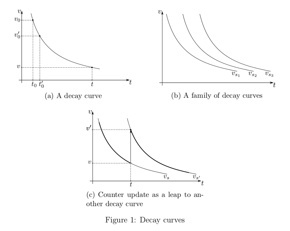
Generally speaking, we do not have a single decay curve, but a family
Let us now see how such a counter should be updated. Let
then this is the value of
Remark
If one wants to count weighted events, the stepwise change should be not by one but by the weight of the event: ![$v'=v+w$]() .
.
It is not yet clear how to find the index of the desired curve, but it will come to light very soon.
2.2 Translational Symmetry
In Fig. 1b decay curves
Mathematically, this property may be written as follows:
that is, the curve
In general, curves may be enumerated any way you like, and you just need to be able to find the index of the new curve during the update operation. But it is more convenient to enumerate them in order so that the index
Remark
Here we introduce the notation ![$\mu(x) := v_0(-x)$]() , which is convenient because the function
, which is convenient because the function ![$\mu$]() increases monotonically. This will come in handy later in Section 2.4 in determining the rate.
increases monotonically. This will come in handy later in Section 2.4 in determining the rate.
Now, the update rule on an event arrival at time
Thus, the update rule appears as
where
This rule looks so simple and universal that it may be taken as the definition. That is how we will define the u-model.
Remark
If the decay function is given by a differential equation of such kind:
then it is always easy to find an invariant for that the property (6) holds.
Indeed, the solution of the differential equation may be written as
Thus we can take![$s = t_0-F(v_0)$]() as an invariant, and the corresponding curve is expressed as
as an invariant, and the corresponding curve is expressed as ![$v_s(t)=F^{-1}(t-s)$]() .
.
then it is always easy to find an invariant for that the property (6) holds.
Indeed, the solution of the differential equation may be written as
Thus we can take
Section 3.1 lists the formal properties that the function
2.3 Absolute and Relative
We may say that
The fact that the update function works with the relative counter value reflects the decay principle: if no events occur, then the absolute value of
2.4 Rate Estimate
For the decay model, the value
Preserving not the letter (from the formula (6)), but the spirit of the decay idea, we construct the rate estimate as a function of a single argument, namely, the relative value of the counter:
It turns out that the u-model approach consists of implementing the following plan (yes, it looks a bit punkish).
- We take some models built from “physical considerations”, and for each of them, we express the update rule through a u-function.
- Then we abstract away from the physical sense, leaving only the bare u-function. Now we can, without worrying about the sense, boldly change the u-function, for example, by choosing a computationally cheaper one.
- Finally, we figure out how to reintroduce meaning, i.e., to construct an adequate estimate of the rate.
- PROFIT!
In order to make this plan possible (the snag, obviously, is only clause 3), some constraints on the u-function would have to be imposed, and now let us try to figure out which ones. The reader, however, may skip these motivational considerations and jump directly to the definition of those constraints (9) on the u-function in Section 3.
2.4.1 A Uniform Stream
Our company studies network traffic, and we may need to count network packets arrivals as items. In this case, they form a stream, and its rate is measured in packets per second (pps). Alternatively, we have to take packet size into account, so the size is considered the weight of an event, and correspondingly, the rate of such a weighted stream is measured in bits per second (bps). It may also be important to distinguish packets by their contents (source and/or destination IP address, port number, protocol, etc.), then we group events by their type and create separate counters for each type.
Since we discuss here how to evaluate the rate of an event flow, we must first formalize the notions of the event and the event stream.
Definition (event). Let us call an event a triple, where
is the event arrival time,
is the event weight,
is the event type, some stream identifier.
Definition (event stream). An event stream is defined as a sequence of events,
. And the events in the stream must be ordered by time:
at
.
In most implementations of event accounting systems, the time is considered a discrete value:
If we are interested only in events as such, e.g., we measure the number of packets in pieces per second, then the weight
Definition (uniform stream). A deterministic uniform streamis defined as follows:
Whereis the stream parameter, i.e., the period between events. Then the rate of such a stream, by definition, is expressed as
.
Now we can express a way to measure the stream rate for any model. Consider a stream of some known rate
We want the stream rate
2.4.2 An Attractor
Studying with concrete examples the behavior of the u-model under the influence of a deterministic stream, we found that (at least for those examples) there is a notion of an attractor, which is somewhat informally described by the following properties.
- For every rate value of the incoming stream
, there exists an attractor, i.e., such a subset of the relative counter values that if any value
ended up in this attractor, then all subsequent values
for
will also end up there. The attractor is an interval
(possibly degenerate, when both ends of it have merged).
- There is convergence: even if the relative value of the counter was outside the attractor, after several updates, it will get there or at least get as close to the attractor as possible.
- There is monotonicity: the position of the attractor depends monotonically on the rate of the incoming stream. That is, both ends of the segment
and
are monotonically increasing functions.
Since we need to judge the rate of the stream by the value of the counter, we need to solve the inverse problem. This is possible due to monotonicity and continuity: there exist functions
Of course, for these properties to be practically useful, first, the segment (attractor) must be short; otherwise, the accuracy will be low, and second, the convergence must be fast, or one will have to wait for a long time before the counter starts to show an adequate value. In any case, for a particular u-model, it is possible to write down the solution explicitly and evaluate the accuracy and speed of convergence.
Let us try to pass from the particular to the general. Now, ask a question: What conditions must be imposed on the u-function for the corresponding u-model to have an attractor with the above properties? An exhaustive answer is given in the next section.
3 Implementation of the U-model
3.1 Definition of the U-model
Let the function
where
Definition (u-model). Consider a counter update method based on the function
having the properties (9), in which the counter updateon
event arrival at timeis expressed by the rule (8):
This way of updating the counter will be called the u-model.
A function
3.2 Rate Measurement
Properties (9) are sufficient to ensure the existence of an attractor and to construct upper
3.2.1 A Strict U-model
We can observe that the conditions (9) do not forbid the case when the increment of the update function converts to zero at some point, that is, when
It is easy to prove that if we take
Definition (strict u-model). If, in addition to the properties (9) functionsand
are strictly monotone on
, then the corresponding u-model will be called strict.
Theorem (fixed point theorem). For a strict u-model under the influence of a deterministic uniform rate stream, a sequence of values
is constant if an additional condition is satisfied: the function
is a compressive mapping, that is,
such that
.
This directly follows from the Banach fixed-point theorem [5], which guarantees the existence and uniqueness of a fixed point in a compressible mapping. Then all terms of the sequence
It turns out that in a strict u-model, the attractor consists of a single point.
In fact, not for all u-models we use the update function is a compressible mapping. For example, the EDecay model has an “almost” compressible update function, as for it, the constant
For example, the following statement holds.
Statement. If at some point in time the counter was in a state where its relative value was, and a deterministic stream of events began to arrive at it, then the sequence of its relative values
tends to some value of
, and the convergence rate is known. In particular, for the EDecay model, the convergence looks like this:
, which, from a practical point of view, allows us to evaluate how quickly and adequately the model responds to changes in the traffic pattern.
3.2.2 A Non-strict U-model
As for discretized models (see Section 3.3), they lose strict monotonicity, so instead of the fixed point theorem, a set of assertions (not given here) that require weaker conditions and give weaker, though still useful, results for rate estimation helps. For the non-strict model, instead of a one-to-one correspondence between the rate of the stream and the relative value of the counter, there is an interval estimate. That is, the attractor is a nondegenerate segment.
Using the proposed methodology, for a given u-model, all that remains is to construct upper
3.3 Discretization
In order to use the u-model in practice, it must be discretized. That is, to make the set of counter states finite and preferably small in size. Why small? We need to keep billions of counters in memory; the more of them, the higher will be the quality of service. Indeed, why should we waste 64 bits per counter when we can do with 16?
Remark
One may go for the trick of complicating the state representation by assuming it as a pair ![$s=(s_{local}, s_{global})$]() , where
, where ![$s_{local}$]() refers to a particular counter, and
refers to a particular counter, and ![$s_{global}$]() is the common part of the state of a whole group of counters. We do use this technique, in particular, to deal with counter overflows, but we do not consider it in this paper.
is the common part of the state of a whole group of counters. We do use this technique, in particular, to deal with counter overflows, but we do not consider it in this paper.
One obvious way to discretize is to select a finite subset of consecutive integers from the continuum of relative counter values and modify the u-function slightly to become an integer.
First, let us construct a function
- it has integer values at integer points:
for
,
- is in some sense close to
:
for
,
- satisfies the conditions (9).
Apparently, this problem may be solved in different ways. Below is one particular way of constructing
The basic idea of this construction is to set the values of
It is more convenient to first construct
where
All that remains is to determine the function
Statement. The functionthus constructed satisfies the conditions (9) and thus defines the u-model.
Remark
Generally speaking, the u-model gets a bit screwed up with this operation (switching from ![$u$]() to
to ![$u^\sqcup$]() ): if it was strict, it ceases to be so after the transformation.
): if it was strict, it ceases to be so after the transformation.
A legitimate question arises: why do we need to add
Remark
There seems to be some meta theorem to claim that, regardless of the way ![$u^\sqcup$]() is constructed at intermediate points, the methodology for constructing the estimates gives the same result.
is constructed at intermediate points, the methodology for constructing the estimates gives the same result.
Now we have a function
How to choose the interval bounds
Take as ![$x_{max}$]() such a number that
such a number that ![$\Delta u^\square(x_{max})=0$]() ,
, ![$\Delta u^\square(x_{max}-1)>0$]() . (By virtue of the condition (9d), such a number exists.) Then the result of the update will never exceed the right bound: for
. (By virtue of the condition (9d), such a number exists.) Then the result of the update will never exceed the right bound: for ![$\forall x\in X^\square$]() we have
we have ![$u^\square(x)\le x_{max}$]() . As for the left boundary, it may be chosen arbitrarily (any
. As for the left boundary, it may be chosen arbitrarily (any ![$x_{min} < x_{max}$]() will do). Indeed, due to non-negativity of
will do). Indeed, due to non-negativity of ![$\Delta u^\square$]() for
for ![$\forall x\in X^\square$]() ,
, ![$u^\square(x)\ge x \ge x_{min}$]() will be satisfied, that is, the result of the update will not exceed the left boundary. Thus,
will be satisfied, that is, the result of the update will not exceed the left boundary. Thus, ![$x_{min}$]() may be chosen based on counter size considerations: the larger the counter capacity, the more left-hand boundary may be moved, and the more accurate the estimate of low-intensity streams will be.
may be chosen based on counter size considerations: the larger the counter capacity, the more left-hand boundary may be moved, and the more accurate the estimate of low-intensity streams will be.
It is this function
Section B of the Appendix shows the discretization of the EDecay model as an example.
4 Examples of U-model Counters
As shown above, the counters introduced in Section 1 (except for linear ones) are represented as u-models. Here we consider them again, now as u-models: first, take the u-function, then construct the estimators.
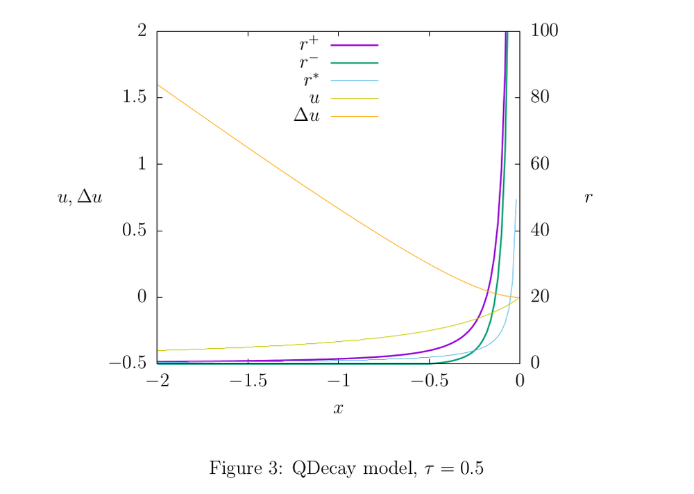
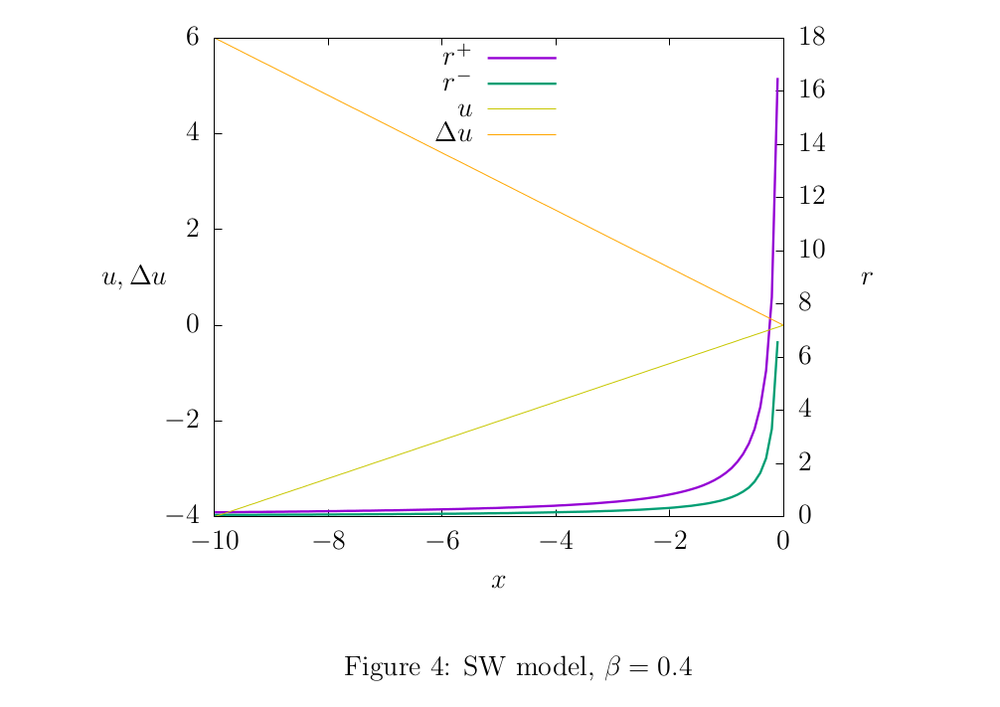
Figures 2,3, and 4 illustrate the properties of the models: shades of yellow show the function graphs
4.1 EDecay
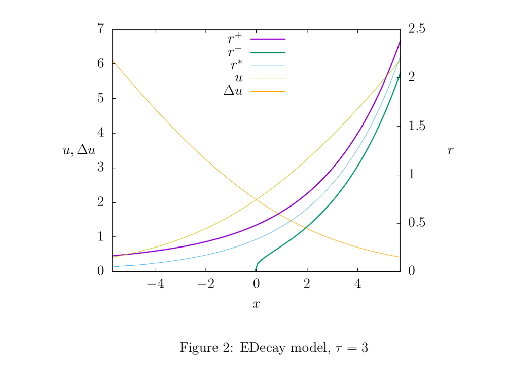
The update rule (1) looks like this:
where
This model has an interesting feature: there is an estimating function
where
4.2 QDecay
The corresponding rule (2) the update function looks like this:
4.3 SW
The update rule (4) is equivalent within the u-model through the update function
A useful property of this model is the computational simplicity of the update function; we can directly write this formula into code without any table approximations.
4.4 Summary Table
Table 1 lists the characteristics of the mentioned models.
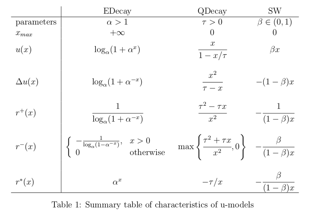
One may notice that for some models, the formula for the lower estimate
In addition to the rigorous rate estimates
Conclusions
The general principles of event counters have been shown in several examples. As a rather universal generalization, the u-model scheme has been proposed. A methodology for constructing rate estimates for any u-model has been proposed.
In addition, a lot of interesting things were left out of the picture.
- Probability Counters. What happens if we replace the
function in the u-model update rule with a random variable that depends on the relative value of the counter?
- Representation and maintenance of large arrays of identical counters. The update and evaluation functions depend on the relative counter value
, where
and
may be in a relatively narrow range of values, while
runs over a wide (potentially infinite) range. How can we make sure that the counters do not overflow?
- Algorithms detecting heavy streams. Individual counters allow us to measure the rate of streams, but how do we organize them to reveal the most intense streams?
Appendix
A Parameterization
All of the counter models discussed in this article are single-parameter. But we use different values in different places to make the formulas look more convenient. Below is a list of quantities that may be equally used as a model parameter, with an indication of their physical meaning and the relationship between them.
-
is the so-called decay constant from the law of radioactive decay [4]
-
,
is a value characterizing the average lifetime in the same model. It is also true that during the time
the amount of decaying matter decreases
times, and the half-life is expressed through
as follows:
.
-
,
.
-
is the smoothing parameter in the EMA [2]
The exponential decay model may be expressed in two ways: through radioactive decay and through EMA smoothing. Here is the relationship between these parameters:.
B An Example of EDecay Discretization
The EDecay model is defined by the following update function:
Consider in Fig. 5 how the update function changes with sampling.
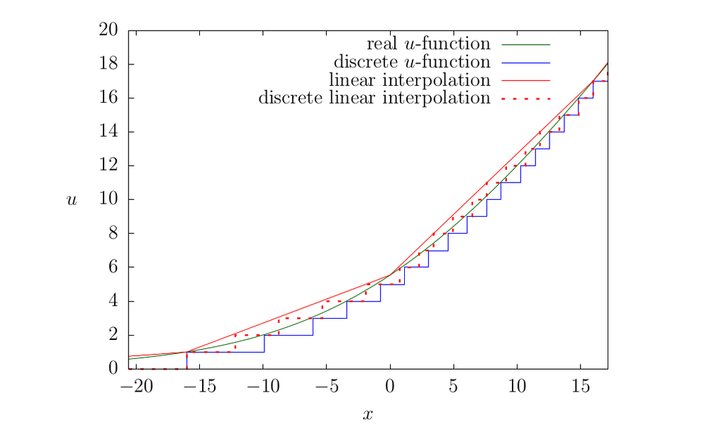
- There is a perfect real-valued update function that exactly exponential decay model (the smooth green line in the graph).
- It has to be discretized for practical applications. It is possible to use a floating-point representation (obviously, it is also discretized, only not uniform) or take an integer representation. In this case, rounding down applies, although it is not crucial (blue line).
- Finally, It is possible to overload the update function even more. In [1] to speed up calculations, it was suggested that instead of calculating the real-valued function with logarithms and exponents, a table approach should be used. It was assumed that the size of the table would be small if a low-digit counter was used. However, nothing prevents us from thinning the table by reducing its size a few more times and implementing linear interpolation. The resulting update function will be slightly different (the red dotted line on the graph).
Of course, as a result of sampling, the update function is distorted, which is not a problem in itself, but we have to take it into account when constructing the rate estimate. In addition, strict monotonicity of the model is inevitably lost, which reduces the accuracy of the estimate. The degree of distortion depends on the parameter
References
[1] Our article about the decay model: https://qratorlabs.medium.com/rate-detector-21d12567d0b5
[2] Exponential moving average: https://en.wikipedia.org/wiki/Moving_average#Exponential_moving_average
[3] Weighted moving average: https://en.wikipedia.org/wiki/Moving_average#Weighted_moving_average
[4] The radioactive decay law: https://en.wikipedia.org/wiki/Exponential_decay
[5] Banach fixed-point theorem: https://en.wikipedia.org/wiki/Banach_fixed-point_theorem
[6] Ayur Datar et al. — Maintaining Stream Statistics Over Sliding Windows — Society for Industrial and Applied Mathematics, Vol. 31, No. 6: http://www-cs-students.stanford.edu/~datar/papers/sicomp_streams.pdf
[7] Our overview of Morris's counters: https://habr.com/ru/company/qrator/blog/559858/
[8] Translational symmetry: https://en.wikipedia.org/wiki/Translational_symmetry