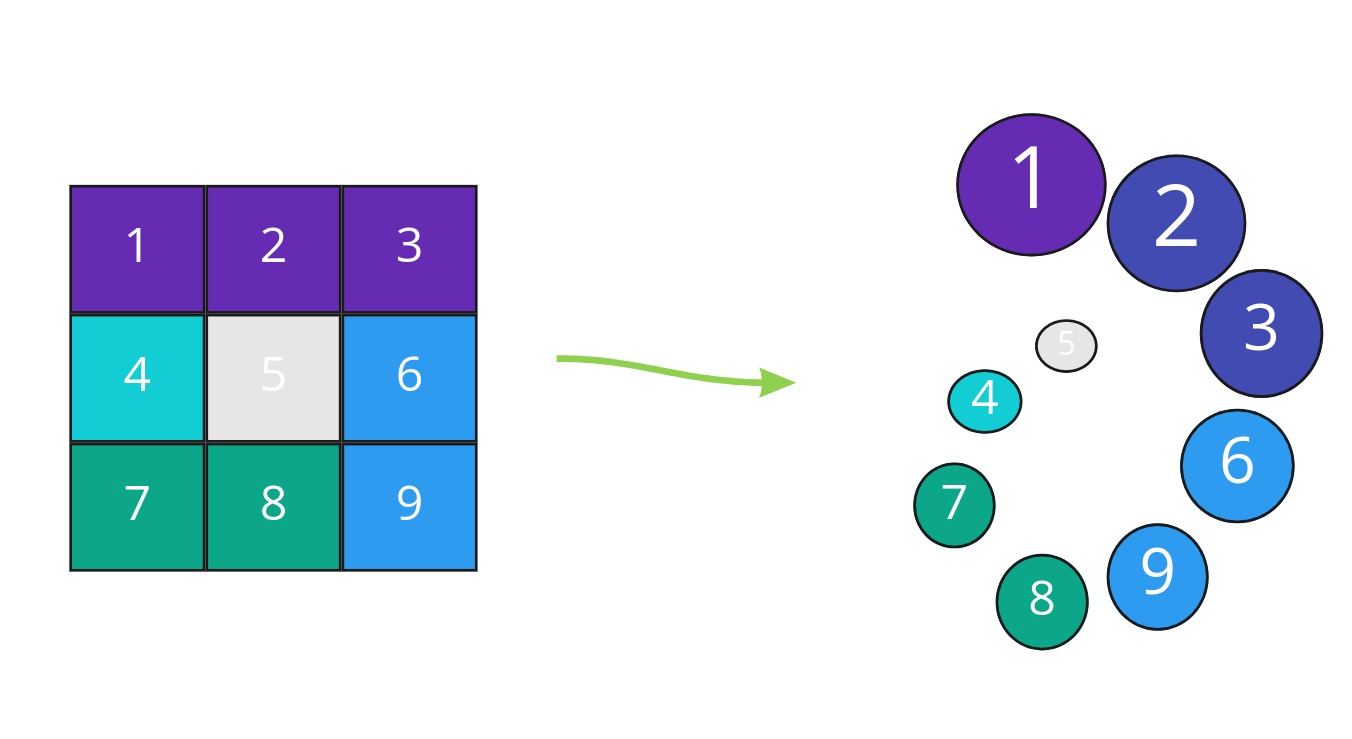
Most solutions to algorithmic problems can be grouped into a rather small number of patterns. When we start to solve some problem, we need to think about how we would classify them. For example, can we apply fast and slowalgorithmic pattern or do we need to use cyclic sortpattern? Some of the problems have several solutions with different patterns. In this article of series Algorithms in Go we consider an algorithmic pattern that solves an entire class of the problems related to a matrix. Let's take one of such problems and see how we can handle it.
How can we traverse a matrix in a spiral order?

We can start with the observation that we are simulating a clock-wise movement and we continue the movement until we exhaust the matrix. How many movements will we have in total? We need to traverse all matrix, therefore the total number of moves will be equal to the total numbers of cells. Ok, then we have a loop condition:
n := len(matrix)    // number of rows
m := len(matrix[0]) // number of columns
// iterate through all cells
for i := 0; i < n * m; i++{
}
What do we do inside the loop?

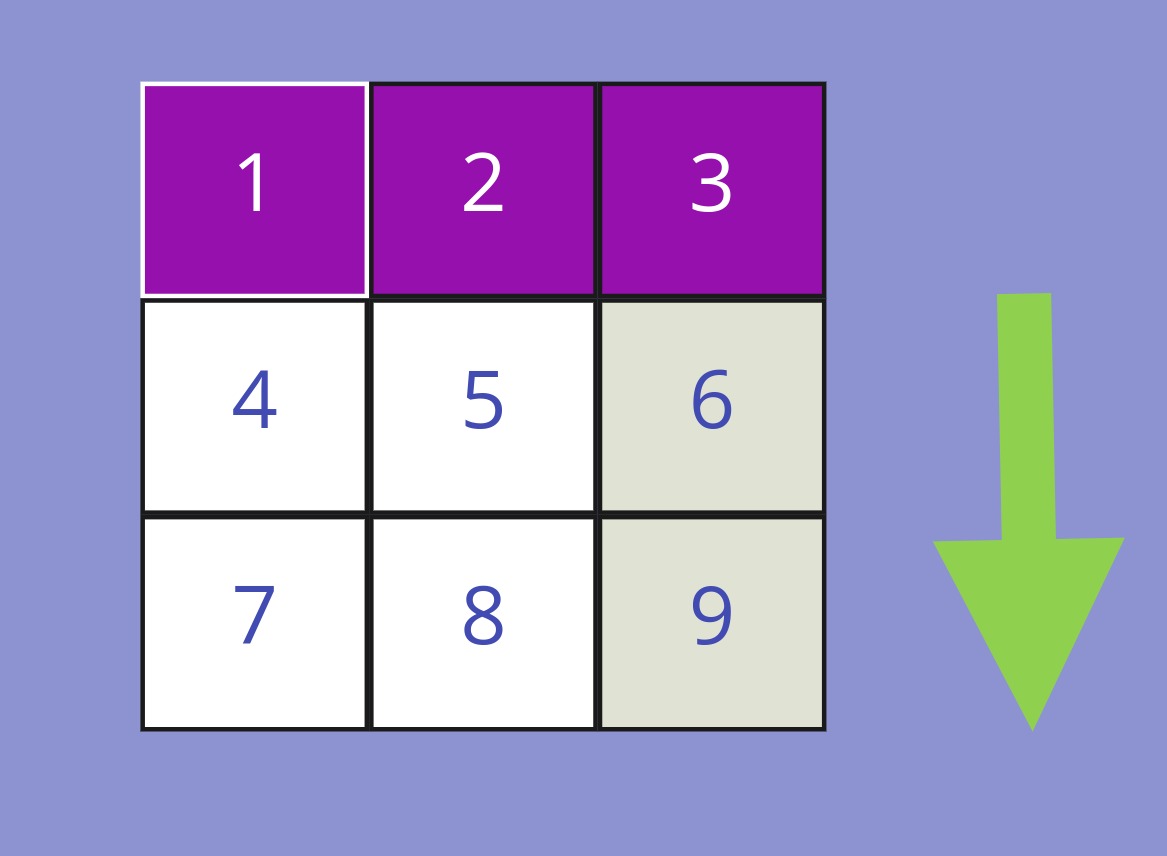
We start with the left movement:

We proceed to the left till we reach the right border of the array, and then change the direction to the downward movement.

We go down until we reach the bottom border and then start to move to the right.

We reach the left border of the array and change the direction the last time and now move upwards.
Let's move :) :
row, col := 0, 0
for i := 0; i < n * m; i++ {
    value := matrix[row][col]
    out = append(out, cell) // save the value
    row, col = applyMove(row, col) // move to the next cell
}
How do we apply to move? We have four possible moves:
// the first value represents the iteration by columns
// the second value represents the iteration by rows
  moves := [][]int{
   {0, 1},  // move to the left column
   {1, 0},  // move down to the lower row
   {0, -1}, // move to the right column
   {-1, 0}, // move to the upper row
  }
If we didn't reach the border we just continue the movement in the current direction. Otherwise, we need to change the move.
When we select the next cell, i.e next row and col values, we check the borders and change the direction if necessary:
func applyMove(row, col int) (int, int) {
    newRow := row + moves[move][0]
    newCol := col + moves[move][1]
    if newRow == -1 || newRow == n || newCol == -1 || newCol == m {
       // change the direction
       move = move + 1
         newRow = row + moves[move][0]
       newCol = col + moves[move][1]
    }
  return newRow, newCol
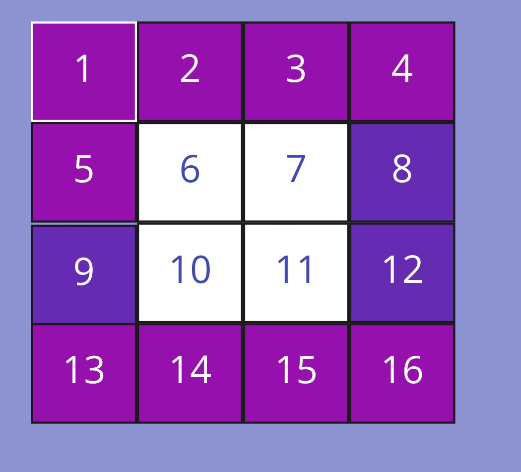
OK, now we can process the first layer of the matrix. How can we generalise the algorithm and process the whole matrix?

We need to stop at the cell with value 1, as we already consumed it, and start the new circle. How do we start the new circle? We change the direction and instead of moving upwards 5 > 1 we go to the left 5 > 6. Therefore, we have a circle in a list of movements and we can help ourselves with a modulo operator:
move = (move + 1) % len(moves)
We also need to save all iterated cells and change the direction if we already processed the cell.
seen[row][col] = true
newRow := row + moves[move][0]
newCol := col + moves[move][1]
if newRow == -1 || newRow == n || newCol == -1 || newCol == m || seen[newRow][newCol] {
 // change the direction
 move = (move + 1) % len(moves)
 row = row + moves[move][0]
 col = col + moves[move][1]
} else {
 row, col = newRow, newCol
}
Full listing:
func spiralOrder(matrix [][]int) (out []int){
    if len(matrix) == 0 {
    return out
  }

  n, m := len(matrix), len(matrix[0])

    // processed cells
  seen := make([][]bool, n)
  for row := 0; row < n; row++ {
      seen[row] = make([]bool, m)
    }

  moves := [][]int{
   {0, 1},  // move to the left column
   {1, 0},  // move down to the lower row
   {0, -1}, // move to the right column
   {-1, 0}, // move to the upper row
  }

  row, col := 0, 0
  move := 0

    applyMove := func() {
      seen[row][col] = true
        newRow := row + moves[move][0]
        newCol := col + moves[move][1]
        if newRow == -1 || newRow == n || newCol == -1 || newCol == m || seen[newRow][newCol] {
           // change the direction
           move = (move + 1) % len(moves)
             row = row + moves[move][0]
           col = col + moves[move][1]
        } else {
       row, col = newRow, newCol
    }
  }

    for i := 0; i < n * m; i++ {
        value := matrix[row][col]
    out = append(out, value)
    row, col = applyMove()
    }

    return out
}
What complexity do we have? We touch every cell only once, so the time complexity is O(n*m). We have an auxiliary matrix seen, therefore our space complexity is also O(n*m).
Can we do better than that? We cannot improve the time complexity as we need to visit all the cells in any case. However, we can think of removing the auxiliary matrix seen. As discussed above we have four movements: left, down, right, up. We need to find a way to limit the range of the movements so we don't slip outside of the borders of the matrix and we don't process the same cell twice. Let's initialize the sentinels.
left := 0
right := m-1
top := 0
bottom := n-1
We start with the left movement and iterate through all cells in the top row. After the iteration we increment top border, as the top row was fully consumed:
for col := left; col <= right; col++ {
    out = append(out, matrix[top][col])
}
top++
Then we go downwards and iterate through all rows from top (which is now equal to one) to bottom inclusive. In this movement we fully consume the right column, therefore we decrease the right border:
for row := top; row <= bottom; row++ {
    out = append(out, matrix[row][right])
}
right--
In the right movement, we consume all cells in the bottom row starting with the right column (which is now equal to last but one column) to the left column inclusive. After the iteration, we have fully consumed the bottom row and decrease the bottom border. Note that we go in the reversed direction, therefore we decrement the value of the current column after the iteration.
for col := right; col >= left; col-- {
    out = append(out, matrix[bottom][col])
}
bottom--
Now, we close the circle and move upwards. We iterate through all the rows starting from the bottom (which is now equal to the last but one column) to the top row (which is now equal to the second row) inclusive. As in the previous movement, we go in the reverse direction and decrease the value of the current row. After the movement, we have fully consumed the left column and can increase the left counter.
for row := bottom; row >= top; row-- {
    out = append(out, matrix[row][left])
}
left++
In this manner, we consume the first layer of the matrix. We continue the iteration till we exhaust the matrix. We need to stop when there are no more columns or no more rows left to process. When left becomes greater than right, we have processed all the columns. When top becomes greater than bottom we have processed all the rows. In either of these two cases, we have no more cells to process. Therefore, our exit condition looks like the following:
for left <= right && top <= bottom {
    // left move
    for col := left; col <= right; col++ {
        out = append(out, matrix[top][col])
    }
    top++

  // downward move
    for row := top; row <= bottom; row++ {
        out = append(out, matrix[row][right])
    }
    right--

  // right move
    for col := right; col >= left; col-- {
        out = append(out, matrix[bottom][col])
    }
    bottom--

  // upward move
    for row := bottom; row >= top; row-- {
        out = append(out, matrix[row][left])
    }
    left++
}
Let's check some edge cases to verify that our algorithm works as intended.
What happens if we deal with a matrix of a single row? Our left move consumes all the cells, our downward move will be no-op as top will be already larger than the bottom. However, our right movement causes the problem as it re-consumes the cells from the last row which is the same as the first row.
In the same vein, in case of a matrix of a single column, our upward movement becomes redundant. Therefore, we need to prevent such movements by the if condition:
if left > right || top > bottom {
    break
}
Therefore, the full listing looks as the following:
left := 0
right := m-1
top := 0
bottom := n-1

for left <= right && top <= bottom {
    // left move
    for col := left; col <= right; col++ {
        out = append(out, matrix[top][col])
    }
    top++

  // downward move
    for row := top; row <= bottom; row++ {
        out = append(out, matrix[row][right])
    }
    right--

    if left > right || top > bottom {
        break
    }

  // right move
    for col := right; col >= left; col-- {
        out = append(out, matrix[bottom][col])
    }
    bottom--

  // upward move
    for row := bottom; row >= top; row-- {
        out = append(out, matrix[row][left])
    }
    left++
}
Now we have time and space complexity both equal to O(n*m).
We can use the same approach to the similar problems of matrix generation or matrix traversal.

