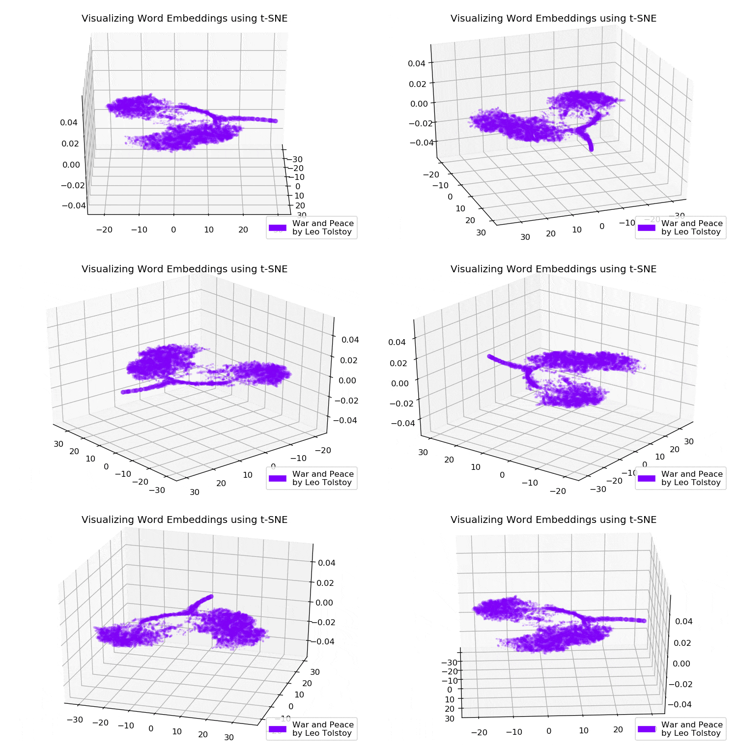
Everyone uniquely perceives texts, regardless of whether this person reads news on the Internet or world-known classic novels. This also applies to a variety of algorithms and machine learning techniques, which understand texts in a more mathematical way, namely, using high-dimensional vector space.

This article is devoted to visualizing high-dimensional Word2Vec word embeddings using t-SNE. The visualization can be useful to understand how Word2Vec works and how to interpret relations between vectors captured from your texts before using them in neural networks or other machine learning algorithms. As training data, we will use articles from Google News and classical literary works by Leo Tolstoy, the Russian writer who is regarded as one of the greatest authors of all time.

We go through the brief overview of t-SNE algorithm, then move to word embeddings calculation using Word2Vec, and finally, proceed to word vectors visualization with t-SNE in 2D and 3D space. We will write our scripts in Python using Jupyter Notebook.

T-distributed Stochastic Neighbor Embedding

T-SNE is a machine learning algorithm for data visualization, which is based on a nonlinear dimensionality reduction technique. The basic idea of t-SNE is to reduce dimensional space keeping relative pairwise distance between points. In other words, the algorithm maps multi-dimensional data to two or more dimensions, where points which were initially far from each other are also located far away, and close points are also converted to close ones. It can be said that t-SNE looking for a new data representation where the neighborhood relations are preserved. The detailed description of the t-SNE entire logic can be found in the original article [1].

The Word2Vec Model

To begin with, we should obtain vector representations of words. For this purpose, I selected Word2vec [2], that is, a computationally-efficient predictive model for learning multi-dimensional word embeddings from raw textual data. The key concept of Word2Vec is to locate words, which share common contexts in the training corpus, in close proximity in the vector space in comparison with others.

As input data for visualization, we will use articles from Google News and a few novels by Leo Tolstoy. Pre-trained vectors trained on part of Google News dataset (about 100 billion words) was published by Google at the official page, so we will use it.

import gensim

model = gensim.models.KeyedVectors.load_word2vec_format('GoogleNews-vectors-negative300.bin', binary=True)

In addition to the pre-trained model, we will train another model on Tolstoy’s novels using Gensim [3] library. Word2Vec takes sentences as input data and produces word vectors as an output. Firstly, it is necessary to download pre-trained Punkt Sentence Tokenizer, which divides a text into a list of sentences considering abbreviation words, collocations, and words, which probably indicate a start or end of sentences. By default, NLTK data package does not include a pre-trained Punkt tokenizer for Russian, so we will use third-party models from github.com/mhq/train_punkt.

import re
import codecs


def preprocess_text(text):
    text = re.sub('[^a-zA-Zа-яА-Я1-9]+', ' ', text)
    text = re.sub(' +', ' ', text)
    return text.strip()


def prepare_for_w2v(filename_from, filename_to, lang):
    raw_text = codecs.open(filename_from, "r", encoding='windows-1251').read()
    with open(filename_to, 'w', encoding='utf-8') as f:
        for sentence in nltk.sent_tokenize(raw_text, lang):
            print(preprocess_text(sentence.lower()), file=f)

On the Word2Vec training stage the following hyperparameters were used:

• Dimensionality of the feature vector is 200.
• The maximum distance between analyzed words within a sentence is 5.
• Ignores all words with the total frequency lower than 5 per corpus.

import multiprocessing
from gensim.models import Word2Vec


def train_word2vec(filename):
    data = gensim.models.word2vec.LineSentence(filename)
    return Word2Vec(data, size=200, window=5, min_count=5, workers=multiprocessing.cpu_count())

Visualizing Word Embeddings using t-SNE

T-SNE is quite useful in case it is necessary to visualize the similarity between objects which are located into multidimensional space. With a large dataset, it is becoming more and more challenging to make an easy-to-read t-SNE plot, so it is common practice to visualize groups of the most similar words.
Let us select a few words from the vocabulary of the pre-trained Google News model and prepare word vectors for visualization.

keys = ['Paris', 'Python', 'Sunday', 'Tolstoy', 'Twitter', 'bachelor', 'delivery', 'election', 'expensive',
        'experience', 'financial', 'food', 'iOS', 'peace', 'release', 'war']

embedding_clusters = []
word_clusters = []
for word in keys:
    embeddings = []
    words = []
    for similar_word, _ in model.most_similar(word, topn=30):
        words.append(similar_word)
        embeddings.append(model[similar_word])
    embedding_clusters.append(embeddings)
    word_clusters.append(words)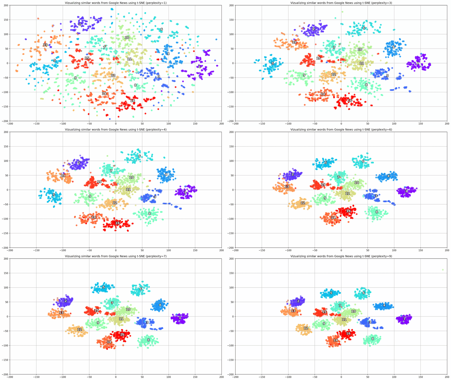

Fig. 1. The effect of various perplexity values on the shape of words clusters.

Next, we proceed to the fascinating part of this paper, the configuration of t-SNE. In this section, we should pay our attention to the following hyperparameters.

• The number of components, i.e. the dimension of the output space.
• Perplexity value, which in the context of t-SNE, may be viewed as a smooth measure of the effective number of neighbors. It is related to the number of nearest neighbors that are employed in many other manifold learners (see the picture above). According to [1], it is recommended to select a value between 5 and 50.
• The type of initial initialization for embeddings.

tsne_model_en_2d = TSNE(perplexity=15, n_components=2, init='pca', n_iter=3500, random_state=32)
embedding_clusters = np.array(embedding_clusters)
n, m, k = embedding_clusters.shape
embeddings_en_2d = np.array(tsne_model_en_2d.fit_transform(embedding_clusters.reshape(n * m, k))).reshape(n, m, 2)

It should be mentioned that t-SNE has a non-convex objective function, which is minimized using a gradient descent optimization with random initiation, so different runs produce slightly different results.

Below you can find a script for creating a 2D scatter plot using Matplotlib, one of the most popular libraries for data visualization in Python.


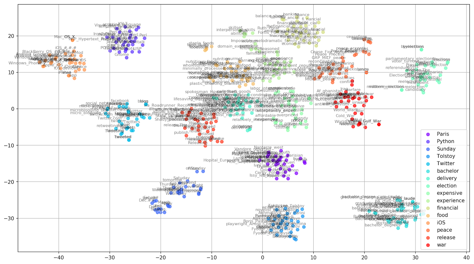
Fig. 2. Clusters of similar words from Google News (preplexity=15).

from sklearn.manifold import TSNE

import matplotlib.pyplot as plt
import matplotlib.cm as cm
import numpy as np
% matplotlib inline


def tsne_plot_similar_words(labels, embedding_clusters, word_clusters, a=0.7):
    plt.figure(figsize=(16, 9))
    colors = cm.rainbow(np.linspace(0, 1, len(labels)))
    for label, embeddings, words, color in zip(labels, embedding_clusters, word_clusters, colors):
        x = embeddings[:,0]
        y = embeddings[:,1]
        plt.scatter(x, y, c=color, alpha=a, label=label)
        for i, word in enumerate(words):
            plt.annotate(word, alpha=0.5, xy=(x[i], y[i]), xytext=(5, 2), 
                         textcoords='offset points', ha='right', va='bottom', size=8)
    plt.legend(loc=4)
    plt.grid(True)
    plt.savefig("f/г.png", format='png', dpi=150, bbox_inches='tight')
    plt.show()


tsne_plot_similar_words(keys, embeddings_en_2d, word_clusters)

In some cases, it can be useful to plot all word vectors at once in order to see the whole picture. Let us now analyze Anna Karenina, an epic novel of passion, intrigue, tragedy, and redemption.

prepare_for_w2v('data/Anna Karenina by Leo Tolstoy (ru).txt', 'train_anna_karenina_ru.txt', 'russian')
model_ak = train_word2vec('train_anna_karenina_ru.txt')

words = []
embeddings = []
for word in list(model_ak.wv.vocab):
    embeddings.append(model_ak.wv[word])
    words.append(word)
    
tsne_ak_2d = TSNE(n_components=2, init='pca', n_iter=3500, random_state=32)
embeddings_ak_2d = tsne_ak_2d.fit_transform(embeddings)

def tsne_plot_2d(label, embeddings, words=[], a=1):
    plt.figure(figsize=(16, 9))
    colors = cm.rainbow(np.linspace(0, 1, 1))
    x = embeddings[:,0]
    y = embeddings[:,1]
    plt.scatter(x, y, c=colors, alpha=a, label=label)
    for i, word in enumerate(words):
        plt.annotate(word, alpha=0.3, xy=(x[i], y[i]), xytext=(5, 2), 
                     textcoords='offset points', ha='right', va='bottom', size=10)
    plt.legend(loc=4)
    plt.grid(True)
    plt.savefig("hhh.png", format='png', dpi=150, bbox_inches='tight')
    plt.show()


tsne_plot_2d('Anna Karenina by Leo Tolstoy', embeddings_ak_2d, a=0.1)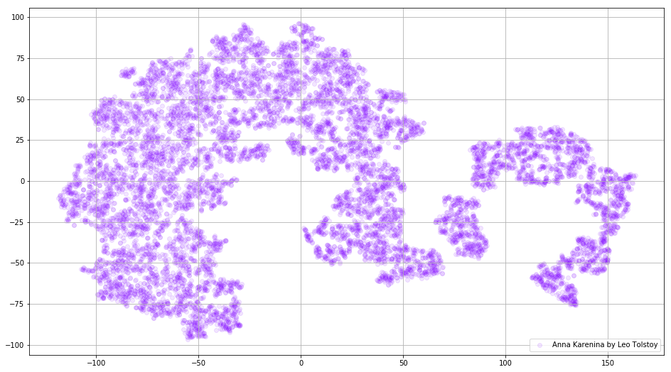

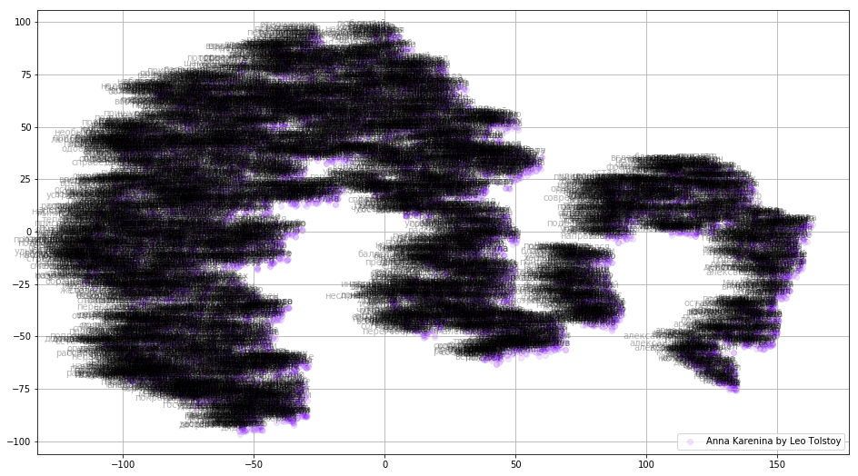
Fig. 3. Visualization of the Word2Vec model trained on Anna Karenina.

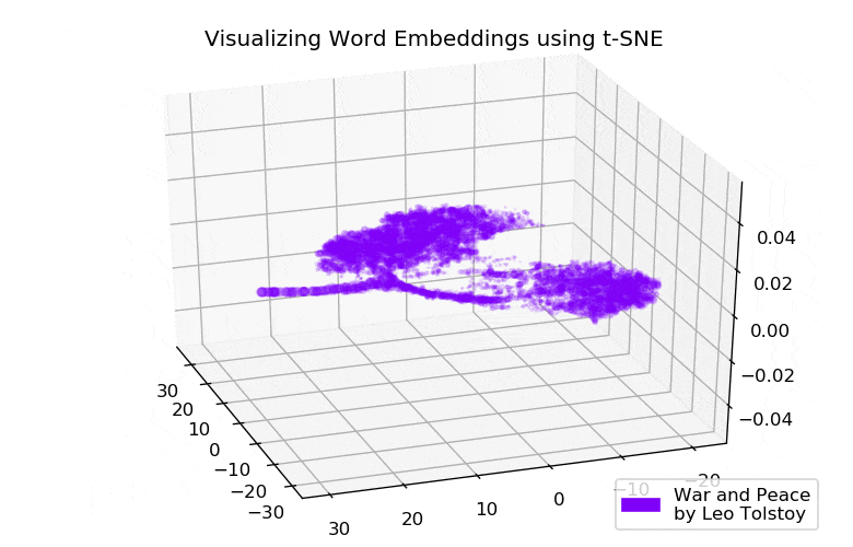
The whole picture can be even more informative if we map initial embeddings in 3D space. In this time let us have a look at War and Peace, one of the vital novel of world literature and one of Tolstoy’s greatest literary achievements.

prepare_for_w2v('data/War and Peace by Leo Tolstoy (ru).txt', 'train_war_and_peace_ru.txt', 'russian')
model_wp = train_word2vec('train_war_and_peace_ru.txt')

words_wp = []
embeddings_wp = []
for word in list(model_wp.wv.vocab):
    embeddings_wp.append(model_wp.wv[word])
    words_wp.append(word)
    
tsne_wp_3d = TSNE(perplexity=30, n_components=3, init='pca', n_iter=3500, random_state=12)
embeddings_wp_3d = tsne_wp_3d.fit_transform(embeddings_wp)

from mpl_toolkits.mplot3d import Axes3D


def tsne_plot_3d(title, label, embeddings, a=1):
    fig = plt.figure()
    ax = Axes3D(fig)
    colors = cm.rainbow(np.linspace(0, 1, 1))
    plt.scatter(embeddings[:, 0], embeddings[:, 1], embeddings[:, 2], c=colors, alpha=a, label=label)
    plt.legend(loc=4)
    plt.title(title)
    plt.show()


tsne_plot_3d('Visualizing Embeddings using t-SNE', 'War and Peace', embeddings_wp_3d, a=0.1)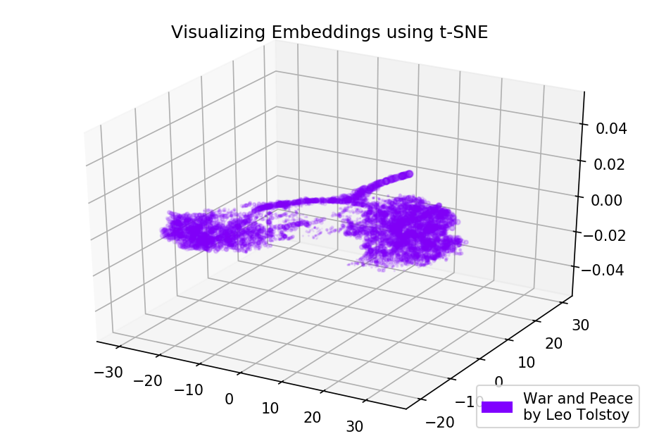

Fig. 4. Visualization of the Word2Vec model trained on War and Peace.

The Results

This is what texts look like from the Word2Vec and t-SNE prospective. We plotted a quite informative chart for similar words from Google News and two diagrams for Tolstoy’s novels. Also, one more thing, GIFs! GIFs are awesome, but plotting GIFs is almost the same as plotting regular graphs. So, I decided not to mention them in the article, but you can find the code for the generation of animations in the sources.

The source code is available at Github.

The article was originally published in Towards Data Science.

References

1. L. Maate and G. Hinton, “Visualizing data using t-SNE”, Journal of Machine Learning Research, vol. 9, pp. 2579–2605, 2008.
2. T. Mikolov, I. Sutskever, K. Chen, G. Corrado and J. Dean, “Distributed Representations of Words and Phrases and their Compositionality”, Advances in Neural Information Processing Systems, pp. 3111–3119, 2013.
3. R. Rehurek and P. Sojka, “Software Framework for Topic Modelling with Large Corpora”, Proceedings of the LREC 2010 Workshop on New Challenges for NLP Frameworks, 2010.